1. Fundamentals of high-efficiency coding

Digitizing a television signal in its original form produces a huge amount of information. For example, digitizing the NTSC signal that is currently used in Japanese broadcasting results in a data rate of 100 Mbps, with a standard definition television component signal and an HDTV production standard signal resulting in about 216 Mbps and 1.2 Gbps, respectively. Transmitting this amount of information, which is at least 1000 times as much as an audio signal, requires a broadband transmission path, and recording it requires large-capacity storage equipment.
A picture signal, however, possesses multidimensional redundancy. In addition to the strong two-dimensional correlation between adjacent picture elements (pels) over space, there is also correlation along the time axis. A good degree of data compression can be expected by using such statistical properties of a picture to eliminate redundant sections.
Against the above background, high-efficiency coding has been researched for many years with the aim of achieving efficient transmission or storage of picture signals (especially television signals) by reducing their redundancy. The following overviews the properties of video signals in conjunction with their supporting role in the design of coding systems, and describes the framework for compression processing using those properties.

[1] Statistical properties of video signals
A great deal of data has been presented in relation to the statistical properties of television signals and other kinds of picture signals, and models of such signals have been constructed on the basis of that data.

(1) Amplitude distribution

Figure 1: Difference-signal distribution between adjacent pels

Figure 2: Measurement of difference-signal amplitude distribution between frames

Due to the ease of measuring the amplitude distribution of a picture signal, many examples of such measurements can be found. It is intuitively clear, however, that such measurements are extremely dependent on the picture itself and can vary greatly according to shooting conditions. For a television signal, moreover, the non-linearity of the picture tube is corrected (gamma correction) at the camera, which means that the amplitude distribution in camera output will be somewhat different from the optical intensity distribution of the original picture. Rigorous modeling is therefore difficult to achieve, but it is possible to use a uniform distribution as a first-order approximation showing the aggregate average of many pictures.
Picture coding is often carried out using difference signals in the picture instead of amplitude itself. This is because the high correlation of the picture signal means that difference in amplitude between (spatially or temporally) adjacent pels is frequently small. Figure 1 shows an example of a difference-signal distribution between adjacent pels and Fig. 2 shows an example of the amplitude distribution of the difference signal in the temporal direction, i.e., between frames. As shown by these figures, the amplitude density function of the difference signal is nearly a double-sided exponential distribution (Laplace distribution) as given by Eq. (1).

(1)

(2) Correlation function and power spectrum
When the statistical properties of picture information g(x, y) are invariable with respect to screen position, that picture information is called "spatially stationary." The autocorrelation function for stationary two-dimensional picture information is defined as follows.

(2)

This indicates the strength of the spatial correlation between two points separated by a displacement of .
Kretzmer was the first to actually measure a picture's autocorrelation function using optical means. Results of that measurement are shown in Fig. 3. Many subsequent measurements exhibited similar behavior. As shown by the figure, the correlation between adjacent pels is normally high despite the fact that correlation differs according to picture content. This characteristic can be approximated one-dimensionally as follows.

(3)

It can also be expressed two-dimensionally as

(4)

or

(5)

Equation (4) is called the "circularly symmetric model" and Eq. (5) the "separable model." We point out here that horizontal and vertical correlation is somewhat stronger than diagonal correlation in ordinary pictures as reflected by structures and natural objects like the horizon. For this reason, the separable model of Eq. (5) is considered to be closer to reality.
For the separable model, we consider a grid-shaped sample and express the correlation function between pels separated by m pels horizontally and n pels vertically as follows, where the interval between sample points is taken to be x₀, y₀.

(6)

A random signal process that satisfies a condition like this is called a first-order Markov process.
While the autocorrelation function expresses the properties of picture information in the spatial domain, power spectral density (referred to as simply "power spectrum" below) expresses picture properties in the spatial frequency domain. The two-dimensional power spectrum of a picture is denoted as and defined as follows.

(7)

It is known that this power spectrum and correlation function constitute a Fourier transform pair according to the Wiener-Khintchine theorem. This means that a signal with high autocorrelation like a picture signal concentrates power in the low-frequency domain. Letting , , and in Eq. (5), the two-dimensional power spectrum becomes after a Fourier transform.

(8)

The above deals with two-dimensional signals like still pictures, but there is also a three-dimensional autocorrelation function derived by Conner and Limb that deals with moving picture signals. In this regard, they created a model of a moving picture signal that considers object speed or the camera's aperture effect, accumulation effect, etc., and derived autocorrelation based on that model. They also showed that spatial correlation along the direction of motion increases as object speed increases, but that temporal correlation decreases.
Miyahara has also measured the spectrum of the inter-frame difference signal. It was found that the autocorrelation function of this signal derived from that measurement deviates slightly from the exponential function of Eq. (3).

Figure 3: Results of measuring the autocorrelation function

[2] Redundancy and compression
As described in section [1], a picture signal generally has high inter-pel correlation and includes many redundant components. Removing these redundant components should make it possible to represent a signal in an optimal fashion and compress information. Redundancy based on the statistical properties described above is called "statistical redundancy," and how to reduce it is the basis for designing a high-efficiency coding process.
Another form of redundancy targeted for reduction by high-efficiency coding is "visual redundancy." This kind of redundancy is based on human visual characteristics such as the following.

- Visibility with respect to resolution in a diagonal direction is lower than that in the horizontal or vertical direction

- Visibility with respect to high-frequency components is lower than that of low-frequency components

- Visibility with respect to moving objects is lower than that of stationary objects

Visual redundancy is used in analog bandwidth-reduction techniques as exemplified by MUSE (Multiple Sub-Nyquist Sampling Encoding). In digital data-compression techniques, statistical redundancy and visual redundancy are cleverly reduced to achieve high compressibility.

[3] Basic coding/decoding process
The basic picture coding/decoding process including picture input and output is shown in Fig. 4. This process begins with an analog/digital converter (A/D) converting the picture signal output from a photoelectric converter such as a camera to a two-dimensional or three-dimensional digital data array. Each element of this array represents a sample of the picture in question and is called a "picture element," or "pel" for short. This data array includes many redundant components, and the source coder can remove nearly all of these redundancies. The data array is passed through a channel coder that adds previously established fixed-redundant components such as error-correction codes to increase the reliability of transmission or of the storage medium. Note that high efficiency coding here generally means source coding.

Figure 4: Basic steps of the picture coding/decoding process

The source-coding process is shown in Fig. 5. The first step in the process is signal conversion. Making use of video characteristics (statistical redundancy), this step converts the signal into data having a distribution as biased as possible, decreases entropy, and extracts only information that must be coded. In principle, this process is not accompanied by distortion. Next, quantization approximates the extracted data to a finite number of discrete levels and decreases entropy even further. This process, on the other hand, is irreversible and accompanied by distortion. It is common, however, to make use of visual characteristics (visual redundancy) to manipulate the data in such a way as to decrease the amount of subjective distortion as much as possible. Finally, in code allocation, the system allocates optimal binary codes to the symbols output by quantization so that the average code length of coded output approaches the entropy of those symbols. This is a reversible process without distortion.
It should be mentioned here that the constituent elements in the above processes are not designed independently of each other, and that there are techniques for combining two constituent elements.

Figure 5: Source-coding process

2. Elemental technologies

[1] Predictive coding
As described above, a picture signal exhibits high correlation and the difference between adjacent pels is generally small. It is therefore more efficient to transmit differences with respect to what has already been transmitted than to transmit the signal directly. This kind of coding system is called "predictive coding" (of which differential pulse-code modulation (DPCM) is nearly a synonym).
To be more specific, a predictive-coding system stores previous pel values that have already been coded in a memory within the coder, and computes a prediction value x' for pel x that is to be input. The system then quantizes the difference x-x' (prediction error), allocates a code to the result, and transmits the code. On the receiver side, the system first generates a prediction-error signal from transmitted codes and then adds that signal to the immediately previous picture signal that has already been decoded to obtain a new picture signal. The function that calculates prediction values is called a "predictor." The In moving picture coding, it is effective to perform prediction based on pels of the prior field or prior frame. These processes are called "inter-field prediction" and "inter-frame prediction," respectively. In this regard, frequently only a small part of the picture displays motion, for example, a scene showing an airplane flying across the sky. In this case, it is most efficient to extract the moving areas from the magnitude of the inter-frame prediction-error signal and to transmit a prediction-error signal only for those areas (called "conditional replenishment"). With this method, however, coding efficiency rapidly deteriorates as moving areas increase. To combat this problem, the motion quantities (motion vector) of a moving object can be estimated by some method and inter-frame prediction performed after compensating for that amount of motion. This method is called "motion-compensation (MC) prediction." Motion estimation methods include the block-matching method and the gradient method, with the former finding widespread use at present.

Figure 6: Example of predictive coding (intra-field prediction)

Figure 7: Principle of motion-compensation prediction

[2] Orthogonal transform coding
In terms of the frequency domain, the fact that an ordinary picture signal exhibits high correlation means that power concentrates in low-frequency components. Accordingly, coding and transmitting the magnitudes (coefficients) of only low-frequency components where power concentrates should make it possible to achieve an overall reduction in the amount of information.
A method called "transform coding" linearly transforms a correlated signal into a signal having as little correlation as possible, and uses the fact that power concentrates in specific transform coefficients to optimize the amount of information allocated to each coefficient. This process results in an overall reduction in coded information.
In actuality, it is common to divide the image into blocks of appropriate sizes and to transmit the picture signal after performing an orthogonal transformation on each block and quantizing coefficients. Various proposals have been made for the transform bases (waveforms) used in orthogonal transform coding, with two well-known ones being the Hadamard transform that is easy to implement in hardware and the Karhunen-Loeve (KL) transform that is most efficient in principle (though not easy to implement). In recent years, however, the discrete cosine transform (DCT) has found widespread use as it can achieve characteristics near those of the KL transform for ordinary picture signals. Its adoption has also been spurred by the growing ease of implementing DCT processes in LSI devices as circuit technologies continue to progress.

(1) DCT

Figure 8: Transform bases

Figures 8(a) and 8(b) show transform bases for DCT of block-length 8 and those for the KL transform of a picture signal approximating a first-order Markov model and having an adjacent-pel correlation of 0.95. As can be seen, these two sets of transform bases are in near agreement. It can also be theoretically shown that the KL transform approaches DCT as the correlation coefficient approaches 1.0 in the first-order Markov model.
Figure 9 shows an example of DCT coding for a one-dimensional sequence of video-signal values. In this process, the video signal is transformed into an array of component magnitudes (coefficients) corresponding to each of the DCT transform bases. In general, the components for the bases expressing low frequency, which are positioned towards the top of the figure, have large magnitudes. A relatively large amount of information is therefore allocated to these components while a relatively small amount of information is allocated to high-frequency components. This makes it possible to represent a video signal with less information overall than is used to represent the original signal sequence. On the decoding side, the video signal is reconstructed by performing a linear summation of the coefficient-weighted transform bases received from the coding side.
Because a picture signal has high correlation in both the horizontal and vertical directions, it is common practice to perform a two-dimensional DCT in these directions using a 8-pel-horizontal by 8-pel-vertical block.
The DCT exhibits nearly optimal characteristics in the sense that it concentrates power in certain coefficients (coefficients corresponding to low-frequency bases), as described above. On the other hand, DCT can also be a cause of picture degradation due to features like block distortion and mosquito noise, as described below.

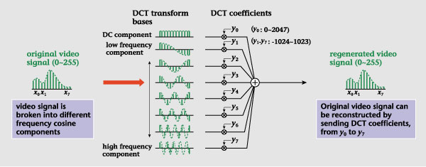Figure 9: Example of DCT coding (1 dimensional process)

(2) LOT

Figure 10: LOT basis area

Coding that performs transformations in units of blocks as in DCT can be a source of visual degradation called "block distortion" in which block structures can be seen in the decoded picture when the DCT is given an insufficient amount of information. To prevent this from happening, methods like the lapped orthogonal transform (LOT) and wavelet transform are being studied. The former transform, which uses bases representing the overlapping of transform bases at adjacent blocks (Fig. 10), is described first.
In LOT, N*N transform coefficients are determined from the pel values of a 2N*2N block, and overlapping of this block with adjacent blocks therefore occurs for N/2 pels at the top, bottom, left, and right. On the decoding side, a 2N*2N block of pels is reconstructed, and the overlapping sections are added on. This process ensures continuity between adjacent blocks and reduces block distortion.
In deriving the bases used in LOT, the bases of overlapped adjacent blocks are assumed to be orthogonal DCT bases. Establishing this condition maintains the key DCT feature of concentrating power. Nevertheless, with LOT and the wavelet transform described below, block-wise discontinuities may occur in the signal targeted for transformation, due to block-by-block processing for motion compensation or other reasons. To solve this problem, overlapping motion compensation has been proposed.

(3) Wavelet transform
In DCT coding, the existence of discontinuities like sharp edges within a block can result in the appearance of ringing artifacts called "mosquito noise" or "corona effects" around those edges. This kind of visual degradation occurs because a local change affects the entire transform block due to the use of transform bases that have the same length from low to high frequencies. The wavelet transform, on the other hand, features a short transform basis length for high-frequency components compared with that for low-frequency components. This lowers the effect of local changes with respect to high frequencies and suppresses the occurrence of mosquito noise.
In frequency analyses such as a Fourier transformation, it is not known where a change in the signal has occurred. The wavelet transform, however, does allow analysis in both the frequency and temporal domains and uses transform bases that are localized in time.
In general, "wavelets" are expressed as a set of functions as in Eq. (9) that can scale by a factor of a (scale transform) or shift by a factor of b (shift transform) the "basic wavelet" function , which is to be localized in either time or frequency.

(9)

Equation (9) can be used to extract time and frequency components from a signal in accordance with parameters a and b in an operation called a "wavelet transform." As a becomes larger, that is, as frequency becomes higher, the width of the waveform becomes smaller, temporal resolution increases, and frequency resolution decreases (Fig. 11).

Figure 11: Wavelet transform

Figure 12 compares the transform bases of the wavelet transform with those of DCT. As mentioned above, the wavelet transform can suppress the spread of high-frequency mosquito noise in areas near object edges or the like where the signal changes sharply. Moreover, in a manner similar to LOT, adjacent transform bases overlap in a wavelet transform and block distortion will not, in principle, appear.

Figure 12: Comparison of transform bases between the wavelet transform and DCT

The wavelet transform can be implemented as a filter bank that recursively divides the low-frequency area, as shown in Fig. 13. In other words, the wavelet transform can be treated as a high-pass filter in which a certain frequency band is extracted and low-frequency components are thinned out in a ratio of 2:1 for another round of filtering. This thinning-out operation is equivalent to extending the previous basis function by two times, and repeating this operation makes it possible to extract low-frequency components from high-frequency components in a stepwise manner.

Figure 13: Implementation of the wavelet transform by a filter bank

[3] Vector quantization
Vector quantization is a method that represents a group of pels in vector form and performs an optimal quantization of that vector. In this method, coding efficiency near the theoretical limit can be achieved by increasing the dimension of the vector. Doing so, however, rapidly increases the amount of coding processing, so a vector dimension of 16 corresponding to a group of 4 horizontal pels * 4 vertical pels is typically chosen as a realistic compromise.
The coding procedure is as follows. The system first divides the image into blocks of 4*4 and compares each block with a previously prepared set of standard pel patterns called a codebook. Then, for each block, the system sends an index value corresponding to the pattern that best approximates that block. On the decoding side, the system reproduces the pattern corresponding to the received index value using the same codebook as the coding side.
Figure 14 compares vector quantization with scalar quantization, which quantizes each pel individually. In particular, Fig. 14(a) shows the result of performing scalar quantization on two pels individually, while Fig. 14(b) shows the manner of quantization that can be achieved by performing a vector quantization that treats x₀ and x₁ as a pair in the form of a two-dimensional vector. Dividing the signal space multidimensionally in this way can reduce overall quantization distortion.

Figure 14: Comparison of vector quantization and scalar quantization

On the other hand, deriving a method for designing a compact and highly general codebook and reducing the amount of quantization computation and required memory are important issues in vector quantization. As a means of dealing with the former issue, the so-called Linde-Buzo-Gray (LBG) algorithms developed by Linde et al. are known. As for the latter issue, it has already been mentioned that because of processing and memory restrictions, a 16-dimensional 4*4 vector is currently considered to be the upper limit. Even at this dimension, however, a huge number of computations are needed to ensure good-quality reproduction. Various solutions to this problem have been proposed. One is the "tree search algorithm" that uses a hierarchically arranged codebook corresponding to the division of signal space into levels to reduce the amount of computation up to the output vector of the final node. Another is "mean-separation normalized vector quantization" that performs vector quantization after first subjecting an input picture signal to mean separation and normalization and then converting it to a standard probability distribution.

[4] Subband coding
The subband coding technique first divides the input signal into a number of separate bands through the use of filters, and then codes the picture of each band individually. Using subbands in this way makes it possible to allocate an appropriate amount of information to each band and to control the frequency distribution of the distortion. In other words, subband coding allows for coding control that considers not only the power spectrum distribution of the picture signal but also the characteristics of human vision. In addition, the ability of forming a hierarchy in the frequency domain means that subband coding can be used as a resolution-conversion technique when transmitting picture signals between systems of different resolutions and as a technique for achieving graceful degradation.
An example of a subband-coding procedure is shown in Fig. 15. On the coding side, the system divides the input signal into separate bands using analysis filters and performs downsampling in accordance with the bandwidths in question. On the decoding side, the system synthesizes the picture after performing upsampling.

Figure 15: Example of a subband-coding procedure

In addition to one-dimensional division, subband division is also capable of two-dimensional division in the horizontal and vertical directions as well as three-dimensional division that includes the temporal direction. Two-dimensional division, however, is the most common.
To raise coding efficiency here, DPCM, orthogonal transform, or other coding methods may be used to code the divided signals. Further division of these signals, moreover, can eliminate spatial redundancy and allows for a configuration that negates the need for orthogonal transform or the like. In this case, either all bands are further divided or only low-frequency signals are recursively divided. A technique that adaptively changes the method of division according to picture content has also been proposed. Coding only by band division features no block distortion as seen in orthogonal transform coding. Similar to LOT, however, it is not highly compatible with adaptive processing in block units, and some sort of measure to deal with this problem is required.
Types of subband filters include the quadrature mirror filter (QMF) and the symmetric short kernel filter (SSKF).

Figure 16: Two-dimensional subband division

[5] Entropy coding
Entropy coding shortens the average code length with respect to the source output having a finite number of symbols. It does this by using occurrence probability to allocate short code words to symbols with high frequencies of occurrence. This is an information-preservation type of coding that uses only statistical properties.

(1) Huffman coding
Given the occurrence frequency of coded objects (here, output values of quantization), Huffman coding minimizes the average code length by allocating codes of optimal code length according to frequency of occurrence.
Taking orthogonal transform coding as an example, the output values of quantizing the coefficients of low-frequency components are large while a high probability exists that the output value of quantizing a coefficient of a high-frequency component is zero. With this in mind, we start from a DC level in a two-dimensional DCT and extract quantization levels by zigzag scanning in the horizontal and vertical directions toward high-frequency components, as shown in Fig. 17. As a result, relatively large values will consecutively appear at the beginning of the scan while the probability that a run of zeroes occurs in the high-frequency area is high. It is therefore efficient in many cases to perform "run-length" coding that codes the length of a run of zeroes. At this point, Huffman coding can be performed in two ways. The first way handles symbols representing a level other than zero and symbols representing run-length in the same coding space, and allocates Huffman codes according to the occurrence frequency of both types of symbol. The second way treats the combination of run-length and the following non-zero level as one symbol, and allocates Huffman codes according to the occurrence frequency of such symbols (two-dimensional Huffman).

Figure 17: Zigzag scanning

(2) Arithmetic coding
The arithmetic coding technique divides the interval [0, 1] on the number line into lengths proportional to the appearance probability of symbols and allocates the symbols in the stream targeted for coding to their corresponding partial intervals. This division process is then repeated, and the number expressing the coordinate of a point in the finally obtained interval as a binary fraction is taken to be the code of that symbol stream. The longer the stream becomes, the closer the average code length gets to entropy.
The main purpose of arithmetic coding is to code binary data, but it can also be used to turn multi-value information sources (like pictures) into binary data. Arithmetic coding expressly for multi-value use is also being studied.

(Dr. Yoshiaki Shishikui)